Utilizing Precalculus Experiences with Graphing Calculators:
A Local Linearity Approach to Calculus

Daniel J. Teague
The North Carolina School of Science and Mathematics
1219 Broad Street
Durham, North Carolina 27715 USA
e-mail: teague@odie.ncssm.edu

Each of the calculus reform projects is experimenting with both content and pedagogy.
By sharing and combining ideas, perhaps we will create introductory calculus courses
that satisfy the competing factions in the calculus debate.

The historical role of calculus in the mathematical preparation of mathematicians, engineers, and scientists is being pitted against the emerging role of calculus in the general education of the informed citizen. For the calculus instructor, these competing roles create a tension between the need to present arguments that are informative and engaging at the level of the student's understanding, and the desire to present arguments that are mathematically rigorous, but perhaps, not as illuminating. For the writer of calculus textbooks, it means deciding whether to present arguments that will convince the students professors meet in their classes or the colleagues they meet in the hall.

The effect of computer technology on the teaching and learning of calculus has been central to this discussion. Students with a strong calculator-based precalculus experience come to calculus with different skills and conceptions of mathematics. It is important to take advantage of these new skills. This paper presents some aspects of the development of calculus at the North Carolina School of Science and Mathematics (NCSSM) which utilize the geometric ideas and understandings students have developed when using graphing calculators in preparatory courses.

Local Linearity

Students who have used graphing calculators extensively in their preparatory courses are familiar with the principle of local linearity. They know from much experience that if they `zoom in' on just about any section of one of the functions they have studied, the function quickly `becomes linear'. Having students begin their calculus course with this experiential base has made a tremendous difference in how we approach the theoretical aspects of calculus.

Calculus adds to this experiential base by explicitly expressing the `zoom line' as the tangent to the curve at x = a,

If the function is indistinguishable from its tangent line in some small region around x = a, then the function is said to be locally linear. The principle of local linearity is closely related to that of differentiability; a function is locally linear at all points at which it is differentiable. By emphasizing the visual, geometric aspect of local linearity and the greatly simplified algebraic operations with linear functions, we can offer students intuitively appealing, convincing arguments to support their understanding of calculus.

The mathematics faculty at NCSSM use the principle of local linearity in its theoretical development of calculus. To illustrate the approach, we consider three important theorems in elementary calculus; l'Hopital's Rule, the product rule for derivatives, and the Fundamental Theorem of Calculus.

l'Hopital's Rule (Weak Form)

The classic approach to this theorem is as follows:
Theorem: Assume that

, that

and

exist, and

.
Then

Proof: .

My students often commented after this development, `I see that its true, but I don't see why its true.' What insight does this derivation give the student? Compare the formal proof above to the less formal argument below.

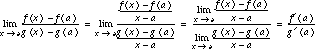
The simplest of all cases is . If f and g are linear, the ratio of ax to bx is always constant for non-zero x,
so the limit is just

Figure 1: Example of f(x) = 5x and g(x) = 2x on [-2,2] and [-0.002,0.002]

With arbitrary functions f and g, the ratio of f(x) to g(x) is not constant, but changes with x. However, if f and g are differentiable at x = 0, they are locally linear near x = 0 with and . If you zoom in on f and g around zero, the geometry gets closer and closer to that of the simple linear case.

If f and g are well approximated by their tangent lines, we can expect near x = 0. This is just the simple linear problem, with .

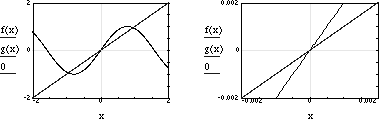
Figure 2: Example with f(x) = sin(2x) and g(x) = x on [-2,2] and [-0.002,0.002]

If we move away from the origin, we have .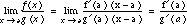

With this argument, students can `see' why l'Hopital's Rule is true. If you zoom in on differentiable functions, they behave locally as if they are linear. As a general approach to questions in calculus, we reduce the problem to its linear approximation, and ask the questions of this simple linear form.

There is more to it than this, of course. Henry Pollak once commented that, `In introductory calculus, you cannot tell the whole truth. If you could tell the whole truth, there wouldn't be a course called analysis.' Given that you cannot tell the whole truth, each of us must decide what parts of the truth to tell. At NCSSM, our effort has been to make the fundamental truths of calculus believable and understandable, and to offer a basis on which to build future work.

The Product Rule

Theorem: Let f and g be differentiable at x = a, and let h(x) =

, then

Proof: . Add and subtract in the numerator so that

Factoring and rewriting, we have

After this presentation, the question from students is, `How would you know what to add if you didn't already know the answer?'

As with l'Hopital's rule, an alternate development begins by considering the linear approximations. If both f and g have derivatives at near x = a, then and .

The function h(x), being the product of f(x) and g(x), can be approximated near x = a . by the product of the two linear approximations, so that .

That there are better quadratic approximations to h is a matter to be taken up later.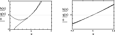

Figure 3: and the quadratic approximation

This product of the linear approximations simplifies to
,
so

for values of x near a. However, at x = a, the approximations are exact, and
,

which gives the product rule

(1)

Our original choice of x = a was arbitrary and depended only on both functions f and g having derivatives at x = a; therefore, the relationship in equation (1) holds for any x where the functions f and g differentiable.

By using the linearity approach, students can derive the product rule themselves, without knowing the result ahead of time. Students learn to use linear approximations as a guide to understanding the behavior of nonlinear functions. In so doing, they have learned more than a result, they have developed a general problem-solving technique through which they can investigate the subject of calculus.

The Fundamental Theorem of Calculus

Rather than approach the fundamental theorem of calculus through an area argument, we utilize the student's understanding of Euler's method as a path to this important theorem. Euler's method is yet another application of linear approximations.

Given a differential equation and an initial condition , Euler's method allows us to generate a sequence of values, that approximate the values of by iterating the equation . The accompanying values of are produced by iterating the equation .

The sequence of values,

,
,

allows us to find approximate solutions to a number of challenging differential equations. However, we can rewrite these expressions to achieve a different purpose. Substituting the expression for y₁ into the equation for y₂ yields

and substituting this expression into the equation for y₃ gives
.

Continuing in this manner, after n iterations an approximation y_n for f(x_n) is given by

.

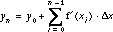Subtracting y₀ from both sides gives .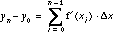

We know that y₀ = f(x₀) while y_n, so the difference y_n - y₀ is an approximation for f(x_n) - f(x₀), the net change in f(x) from x₀ to x_n. This gives
.

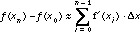As goes to zero, y_n approaches f(x_n), so that gets closer to the actual value of f(x_n) - f(x₀). Indeed,

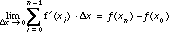(2)

where and x_i = x_i_-1 + .

We then define the definite integral 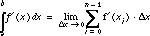, where a is x₀ and b is x_n. Since the right side of equation (2) is the net change in f(x) from x = a to x = b, which is f(b) - f(a), the definite integral on the left side of this equation also equals the net change in f(x), so that

Conclusion

Thirty years ago, the calculus curriculum was designed for mathematics, engineering, and science majors, whose preparatory courses, from Algebra I to Precalculus, were explicitly organized to prepare them for that experience. To meet the needs of students in today's world, the precalculus curriculum must do more than lay the groundwork for calculus. Calculus itself is no longer a course only for students preparing for careers in mathematics, engineering, and the sciences. As teachers of mathematics, we must seek new and more effective ways to motivate and teach to an ever-changing population the principles of calculus needed to fulfill roles in business, industry, and as intelligent citizens. The fundamentals of calculus remain the same, but the students to whom we teach calculus do not. The techniques described here have been shown to work well with students who enter the calculus class experienced with graphing calculators. In many ways, these students are better prepared for calculus than their predecessors. In other ways, they are less well prepared. To teach calculus effectively, we must know our students. We must understand what skills they have and what skills they lack, and devise approaches that take advantage of their abilities.

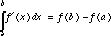
The linearity approach falls short of the criterion for rigor desired by many, but is in line with Ron Douglas's comment in Toward a Lean and Lively Calculus that `I believe that students should learn that the fundamental notion of the differential calculus is how effective linear and quadratic approximation is for studying nice functions and how this can be used to study systems that change.' Students can reduce the problem to the linear approximation, `follow the lines', and make a conjecture about how well the behavior of the linear model represents the behavior of the function. For students who demand formal proofs, the linearity approach offers an important first step. Rather than be presented with a theorem as a pre-packaged statement, the students will make conjectures based on the behavior of the linear approximations that they must either fully justify or reject. This presents in a much more realistic context the process of mathematical investigation.

References

Bartkovich, Kevin, et al, Contemporary Calculus Through Applications. Providence, Rhode Island: Janson Publications, 1995.

Douglas, R. G., "Opening Remarks at the Conference/Workshop on Calculus Instruction, in Douglas, R. G. (ed), Toward a Lean and Lively Calculus, (MAA Notes Number 6). Washington, DC: Mathematical Association of America, 1987.

ICME8 - WG13 - 02 JUL 96

[Next] [Previous] [Top]

Generated with CERN WebMaker