[Next] [Previous] [Top]
Promoting Changes in the Curriculum by Means of Dynamic Technologies - An Example
Abraham Arcavi - Nurit Hadas
Department of Science Teaching
Weizmann Institute of Science - Rehovot - Israel
Introduction
There are several possible approaches in which dynamic computerized environments play a significant, and possibly unique, role in supporting innovative learning trajectories in mathematics, in general, and particularly in geometry. These approaches are indeed tainted by the way one views mathematics and mathematical activity.
In this paper we briefly describe our approach (or credo, if you will) and a problem situation to exemplify it. On that basis, we then discuss the ways in which we believe the mathematics curriculum, and ensuing classroom practice, can radically depart from tradition.
Rationale
Dynamic computerized environments constitute virtual labs in which students can play, investigate and learn mathematics. The following are some of the characteristics nurtured by such labs, provided they are accompanied by suitable curriculum materials.
Visualization
`Visualization generally refers to the ability to represent, transform, generate, communicate, document, and reflect on visual information' (Hershkowitz, 1989). As such it is a crucial component of learning geometrical concepts. Moreover, a visual image, by virtue of its concreteness, it `is an essential factor for creating the feeling of self-evidence and immediacy' (Fischbein, 1987, p.101). Therefore, it `not only organizes data at hand in meaningful structures, but it is also an important factor guiding the analytical development of a solution.' (ibid.) Dynamic environments, not only enable students to construct figures with certain properties and thus visualize them, but also allow for `continuous' transformations of those constructions in real time according with what the user decides. This dynamism contributes further to the strength of the visual experiences.
Experimentation
While playing with technological environments students learn to experiment, and `to appreciate the ease of getting many examples..., to look for extreme cases, negative examples and nonstereotypic evidence...'(Yerushalmy, 1993). They do so by looking, measuring, comparing and changing (or even distorting) figures. The information obtained in this way is the basis for stating generalizations and conjectures. Some of those conjectures can be dismissed by further experimentation, others require confirmation which some students may tend to accept on the basis of nothing but more positive evidence. Some authors (e.g. Laborde, 1993) have warned about the dangers of such `inductivism'. Experimentation of the kind described above may enhance (or even contribute to develop) the tendency of many students to content themselves with the accumulation of positive empirical instances as evidence or `proof' of an assertion. Thus, experimentation in itself may not be enough, and this leads us to the next important characteristic.
Surprise
It is unlikely that students will fruitfully direct their own experimentation from the outset. Curriculum activities, such as problem situations, should be designed in which students are invited to engage. The kinds of questions they are asked can play significant roles in the depth and intensity of a learning experience. One significant type of question is to require students to make thoughtful predictions about the outcome of a certain phenomenon at stake or a certain action they take within the technological environment. Making thoughtful and explicit predictions can a) nudge students to be more clear about how they envision the situation they are working on, b) make students more committed to the situation and thus be more careful on the way they think about it, c) create expectation and motivation towards the actual experimentation. For that to occur, the outcome of the activity should not be immediate; moreover it would be desirable if it is counter-intuitive, such that its disparity with explicitly stated predictions generates surprise and puzzlement. In other words, predictions set the scene for the subsequent questioning by the students themselves, and thus enhance the chances for meaningful learning.
Feedback
Notice that a surprise arises from the gap between an expectation and the outcome of an action. Thus the feedback does not consist of a low mark or a reprimand, rather it is provided by the environment itself, which re-acted as it was requested to do. Such direct feedback is potentially more effective than the one provided by a teacher, not only because of its affective underpinnings (lack of value judgment), but also because it may provide actual clues for revising the prediction and further re-thinking on the situation.
Need for proof and proving
Dreyfus and Hadas (in press) argue about (and exemplify) how one can capitalize on student surprises, of the kind described above, in order to instill the need for proof. Following a surprise, many students may require a proof, possibly not by stating that in so many words, but by demanding an answer to their `why'.
The engineering of successful tasks (appropriate for dynamic environments), which lend themselves well to develop surprises and subsequent demands for proof, should take into account something else as well. The proof, namely the answer to the `why', should arise from the observations, or the re-visions of the experimentation process itself. In other words, the experimentation should provide the seeds for the argumentation which helps to proof an assertion. In this way the dynamic environment really supports the `closing of the circle', and thus may promote a meaningful and unique learning outcome.
Intramathematical connections
The Geometry Inventor (1994), one of the dynamic geometry environments available today, offers a window in which Cartesian graphs may be drawn to represent relationships between two variables, concurrently with the occurrence of the changes in those variables. Thus a geometrical phenomenon can be observed as changing dynamically either by looking at it or by watching a Cartesian representation of the changes of two variables of the situation. In this way boundaries between mathematical sub-disciplines are blurred. Moreover, students have an opportunity to appreciate that by confronting the geometrical situation with graphical representations of it, one may enhance the understanding of the situation via the representation and vice versa (Arcavi and Nachmias, 1989).
The nature of mathematical objects
Students usually meet static graphic or symbolic depictions of functions. By being static, these representations, seem to betray a fundamental idea of the dynamism at the core of this concept: change and variation. By seeing, how a graph is being created in real time as describing a situation which is changing in front of our eyes, the technology has the potential to make perceptible the idea of change and variation, its range, and its quality (increase, decrease, expected extrema, etc.).
In the following we analyze a problem situation which, we believe, illustrates and substantiates the claims made above. The description includes the situation itself, its implementation in the Geometry Inventor, anecdotal data from classrooms, and an analysis and discussion of the educational significance and implications.
The problem situation
The first step consists of building on the `drawing board' (of the Geometry Inventor), two 5 units long segments, in such a way that they are contiguous (share one end point) but not collinear. Joining the two other end points, produces an isosceles triangle.
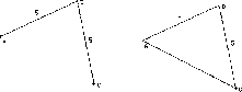
Figure 1
By dragging, for example, the vertex C, we obtain more isosceles triangles whose equal sides are 5.
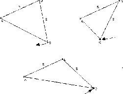
Figure 2
The effect of the continuous and dynamic variation sets the scene for the question: what changes and what stays the same? Students have no difficulty in pointing to the equal sides as the given constants and they mention the most obvious variable: the third side. When required to point to more variables, they also mention the angles and the area of the triangle.
The next step is to look at some of these changes and establish their range. For example, by dragging the vertex C, it is easy to see the limits, namely the minimum and maximum length for AC (0 and 10 respectively, see Figure 3).
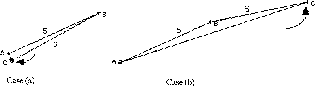
Figure 3
We then turn the attention to the variation of the area as a function of AC. By looking again at the dynamic changes, it becomes apparent that the minimum area is 0 (in the case in which AC is 0), it then increases, but at some point it starts to decrease until it reaches again 0 when AC becomes 10. The next question follows quite naturally: predict when the area reaches its maximum value. In order to have some more experiential basis for the prediction, we suggest to first play with changing the triangle and to get a visual feeling for a maximum area.
We heard different predictions in the classrooms in which we tried this problem. One answer consists of showing (hand waiving) one or more triangles which look like having a maximum area and saying `the largest triangle is one of these'. Another answer, more frequent among teachers with whom we tried this problem, points to the equilateral triangle as being the one with largest area (namely the triangle in which AC is also 5). One can speculate here that their perception of largest area as seen on the screen is misdirected (or overruled) by what they know from allied but yet different situations (e.g. isoperimetric problems).
Given the medium, it is natural that predictions are given in geometrical terms (by way of characterizing the triangle), rather than by giving a numerical value for AC or the area.
All predictions are respectfully treated (the correct one is the least common), and we direct the work back to the `drawing board' for further checks and feedback. At this time, we suggest to introduce measurements, which dynamically change in real time with the changes in the triangle. Measurements play a significant role in providing useful feedback (and specially counterexamples). In the following (see Figure 4) we illustrate how the screen might look like in two discrete shots of the dynamic changes, when measurements are introduced.
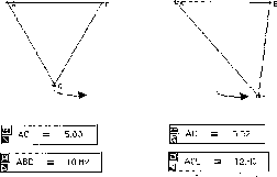
Figure 4
By dragging C `beyond' the equilateral triangle, one can disconfirm the conjecture that it is the one with the maximum area. One notices that the values increase beyond 12, towards 12.4, 12.5 and then begin to decrease. The surprise caused by the disconfirmation of the `equilateral triangle conjecture' sets the scene for the working on the `why', or in this case, the `why not'.
Elaborating the answer may be a matter of the classroom dynamics. It can be aided by hints, such as, `how does one calculate the area of a triangle?' Recalling the half-the-base-times-the-altitude formula is a step further. However, if one chooses AC as the base it is difficult to see anything because both the base and the altitude vary (Figure 5).
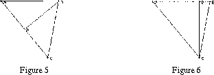
Therefore, we suggest to try to choose another side as the base. For example, AB, in which case the altitude is as shown in figure 6.
We discuss the advantage of this choice over the previous one. Here the base is fixed (5 units) and only the altitude changes. By dragging C again, one is able to `see' not only the correct answer, but the proof as well: the area will be maximum, when the altitude is. We can now vary the triangle to conclude when will that happen.
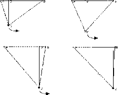
Figure 7
We now have a geometrical explanation: the triangle DBC is right-angled, thus the leg DC is less than the hypotenuse BC, namely less than 5. DC, the altitude of ABC, will be maximal when it coincides with a side (BC), namely when ABC is right-angled.
Moreover, this also explains the 12.5 value for the maximum area (half the base times the altitude is 5x5/2).
To summarize so far, the situation started by visualizing a family of isosceles triangles with equal sides of fixed length, then changing dynamically from one triangle to another, observing variation and making predictions about them. The predictions lead to a surprise, which in turn raised the need for the why (or why not). The answer to that why was induced by further experimentation which produced both the right answer and its justification.
At this point, we turn to a Cartesian representation of the situation. We ask to predict how a graph of the variation of the area would look like as AC changes? (or, if you will, as a function of AC). By placing the values for AC on the x axis, students usually notice that they will be looking at the interval [0,10], and at the interval [0,12.5] on the y-axis. Since the area increases up to a maximum and then decreases to zero, most students predict the graph to be like a parabola. Again, the technological tool enables us to try it and thus step back from giving direct feedback on the prediction. The tool has a graphing window, which, after matching variables to axes and setting appropriate scales, draws a graph in real time. Figure 8 shows a snapshot of what happens dynamically on the screen.
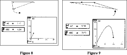
After dragging C, Figure 8 turns into Figure 9.
In spite of having seen that the maximum value for the area is not at the middle of the range (AC=5), students are usually surprised by the asymmetry of the graph. This is because seeing the representation of the phenomenon is quite another thing than seeing the phenomenon itself. Again, here the surprise can drive the search for an explanation. The activity now consists in reinterpreting the graph as a descriptor of the situation by looking at questions such as: what would it mean for the graph to be symmetrical? Where would its maximum be? and so on. In answering these questions raised by the graphical representation of the situation, one has to review in a different light, or reorganize, what was found so far.
Notice that until now, the exploration of the situation had two main phases: the situation itself (i.e. moving around one vertex of the variable triangle and noticing properties) and the graphical representation of the situation (interpreting the graph as a faithful descriptor of the situation and identifying the findings in it). At this point we suggest to investigate the symbolic representation.
The symbolic phase, if undertaken as the last phase, may have a greater significance once one knows what to expect from the symbols as other descriptors of the situation. In other words, if one is to build a symbolic expression for the variation of the area of the isosceles triangle in terms of its variable side, it is expected that the expression will:
a) be 0 when AC is 0 or 10,
b) increase to a maximum and then decreases
c) have its maximum at 12.5
and so on.
Thus, when calculated, Area =  , one can check, by substitution and simple trials, whether it yields what it is expected to. If one goes further and studies the function with more advanced tools (e.g. derivatives) one has on the one hand a background against which to check the results, and on the other hand an illustration about how symbols `speak', namely how they yield the information already obtained. In such a learning trajectory, knowledge of the situation may render symbolism less opaque and more meaningful.
We suggested to explore here a particular function for the area. Obviously one can explore others, for example, the area as a function of the angle between the equal sides and investigate similar issues, like the symmetry of the graph, and yet preserve the same approach (experimentation, surprise, proof, etc.).
The above is just one example of a whole set of problems we are now engineering for use in classrooms.
Educational implications
The above problem and its underlying philosophy imply changes in the curriculum and in the way classroom practices are implemented. The main changes are the following.
- Mathematics incorporates an empirical component. Students are led to explore, to play with many particular cases, to induce dynamic changes and to observe. Intelligent observation not only may add insight and meaning, it may also serve as the basis for proving and further exploring.
- Exploration and conjecturing do not require a teacher whose role is to confirm or judge the conjecture. The teacher becomes a guide who poses the appropriate questions at the appropriate moments. For example, the teacher requests predictions which force students to take a stance on the problem, be explicit about the why (or why not) of what they see. The teacher's role also consists in bringing back the prediction both in cases when it is confirmed or dismissed, and ask `why'.
- Making sense of a situation while playing with the situation itself first, and then by interpreting its representations (graphs, symbols), enhances both the understanding of the situation and of the representations. The concept of function, which models the situation, recovers its dynamism, since its graphical representation is being created in real time as it describes the phenomenon.
Moreover, symbols, which are usually regarded as meaningless, can expected to `convey' a certain meaning, and thus are used and inspected in a different, deeper, way. Also, representations are now seen as ways in which the same information can be encoded, each with its strengths and weaknesses.
- Traditional boundaries between mathematical sub disciplines are blurred. Geometric explanations can be looked upon by interpreting graphs and symbols. One sub-discipline serves as the model for the other, and students can learn to look for consistencies and connections among them.
In summary, the above example shows one possible way in which technology can promote significant changes in the way students learn and teachers teach. We still need, beyond our limited experience, to engage in further research and engineering in order to substantiate more what seems to be a very fruitful direction.
References
Arcavi, A. and Nachmias, R. (1989) `Re-exploring familiar concepts with a new representation'. Proceedings of the 13th International Conference on the Psychology of Mathematics Education (PME 13), Paris, 1989, V.1, pp. 77-84.
Dreyfus, T. and Hadas, N. (In press) `Proof as answer to the question why'. ZDM.
Fischbein, E. (1987). Intuition in Science and Mathematics: An Educational Approach. Reidel.
Geometry Inventor (1994). Logal Educational Software and Systems Ltd.
Hershkowitz, R. (1989). `Psychological Aspects of Learning Geometry'. In Nesher, P. and Kilpatrick, J. (Eds.) Mathematics and Cognition: A research Synthesis by the International Group for the Psychology of Mathematics Education. Cambridge University Press, pp. 70-95.
Laborde, C., (1993). `The Computer as Part of the Learning Environment: The Case of Geometry'. In Keitel, C. and Ruthven,K. (Eds.) Learning from Computers: Mathematics Education and Technology. Springer, NATO ASI Series F 121, pp. 48-67.
Yerushalmy, M. (1993). `Generalization in Geometry'. In Schwartz, J.L., Yerushalmy, M., and Wilson, B. (Eds.) The Geometric Supposer, What is it a Case of?. Lawrence Erlbaum Assoc., pp. 57-84.
ICME8 - WG13 - 02 JUL 96
[Next] [Previous] [Top]
Generated with CERN WebMaker